Statistics - Markov Chain Monto Carlo Methods

 Markov chain Monte Carlo (MCMC) methods
-  MCMC methods are used to approximate the posterior distribution of a parameter of interest by random sampling in a probabilistic space.
- so, what is posterior distribution - In Bayesian statistics, the posterior predictive distribution is the distribution of possible unobserved values conditional on the observed values.
- In statistics, Markov chain Monte Carlo (MCMC) methods comprise a class of algorithms for sampling from a probability distribution. By constructing a Markov chain that has the desired distribution as its equilibrium distribution, one can obtain a sample of the desired distribution by observing the chain after a number of steps. The more steps there are, the more closely the distribution of the sample matches the actual desired distribution.

Some of the advantages of MCMC
- Markov chain Monte Carlo (MCMC) algorithms used in Bayesian statistical inference provide a mathematical framework to circumvent the problem of high-dimensional integrals and allow the likelihood function to be conditional on the unobserved variables in models, simplifying and expediting Bayesian parameter estimation
- Bayesian approach using Markov chain Monte Carlo(MCMC) is that the researcher can replace the unobserved variables by simulated variables, relieving the burden of evaluating the likelihood function unconditional to the unobserved variables to allow a focus on the conditional likelihood function. In many cases, this makes Bayesian parameter estimation faster than classical maximum likelihood estimation
- Avoids many of the approximations used by the frequentist method, improving the parameter estimation and model fit

One of the central aims of statistics is to identify good methods for fitting models to data. One way to do this is through the use of Bayes’ rule: If y is a vector of k samples from a distribution and $z$ is a vector of model parameters, Bayes’ rule gives

                                                           p(z/y)=p(y/z)p(z)/p(y)

Here, the probability on the left, p(z/y) — the *posterior* — is a function that tells us how likely it is that the underlying true parameter values are z, given the information provided by our observations y over some variables x.

Note that if we could solve for this function, we would be able to identify which parameter values z are most likely — those that are good candidates for a fit. We could also use the posterior’s variance to quantify how uncertain we are about the true, underlying parameter values.

Bayes’ rule gives us a method for evaluating the posterior: We need only evaluate the right side of the equation above. We need to evaluate:

p(y/z) — This is the probability of seeing outcome y at fixed parameter values z. Note that if the model is specified, we can often immediately write this part down. For example, if we have a Normal distribution model, specifying z means that we have specified the Normal’s mean and variance. Given these, we can say how likely it is to observe any y.

p(z) — the *prior*. This is something we insert by hand before taking any data. We choose its form so that it covers the values we expect are reasonable for the parameters in question. This is our "wild guess", our *belief*.

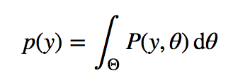
p(y) — the *evidence* (in the deonominator), i.e. the evidence that the data y was generated by this model. Notice that this doesn’t depend on z, and so represents a normalization constant for the posterior.

But p(y) can sometimes be difficult to evaluate analytically. We can compute this quantity by integrating over all possible parameter values, using the law of total probability (we are used to seeing it as a sum $\Sigma$ for discrete variables, this is just its generalization to continuous variables):

This is the key difficulty with Bayes formula -- while the formula looks innocent enough, for even slightly non-trivial models we cannot evaluate it easily. So we need a little help from our computer friends.

**Monte Carlo sampling** is one of the most common approaches for computers to help us.

The idea behind Monte Carlo is to take many samples z_i from the posterior. Once obtained, we can approximate population averages by averaging over the samples.

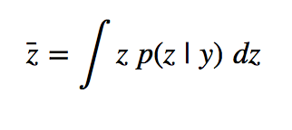
For example, the true posterior average  

can be approximated by the sample average 

By the law of large numbers, the sample average is guaranteed to approach the distribution average as N -> Infinity. This means that Monte Carlo can always be used to obtain very accurate parameter estimates, provided we take N sufficiently large and that we can find a convenient way to sample from the posterior.

Follow and Subscribe:

https://twitter.com/vaishalilambe

https://www.youtube.com/user/vaishali17infy/

https://github.com/vaishalilambe