Distributions 

The distribution of a statistical data set (or a population) is a listing or function showing all the possible values (or intervals) of the data and how often they occur. When a distribution of categorical data is organized, you see the number or percentage of individuals in each group. When a distribution of numerical data is organized, they’re often ordered from smallest to largest, broken into reasonably sized groups (if appropriate), and then put into graphs and charts to examine the shape, center, and amount of variability in the data.

The world of statistics includes dozens of different distributions for categorical and numerical data; the most common ones have their own names. 

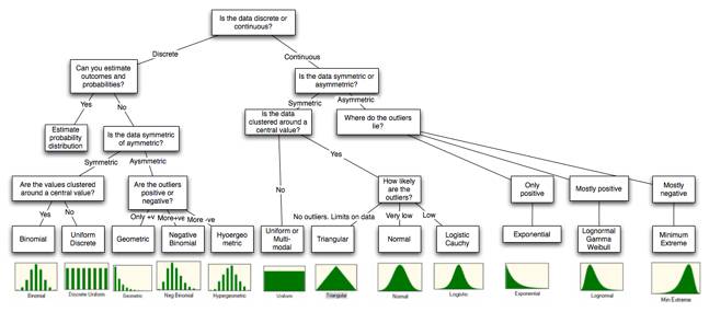
Is the data discrete or continuous?

The first and most obvious categorization of data should be on whether the data is restricted to taking on only discrete values or if it is continuous. 

With discrete data, the entire distribution can either be developed from scratch or the data can be fitted to a pre-specified discrete distribution. With the former, there are two steps to building the distribution. The first is identifying the possible outcomes and the second is to estimate probabilities to each outcome. If it is difficult or impossible to build up a customized distribution, it may still be possible fit the data to one of the following discrete distributions:

1. Binomial distribution 

The binomial distribution measures the probabilities of the number of successes over a given number of trials with a specified probability of success in each try. In the simplest scenario of a coin toss (with a fair coin), where the probability of getting a head with each toss is 0.50 and there are a hundred trials, the binomial distribution will measure the likelihood of getting anywhere from no heads in a hundred tosses (very unlikely) to 50 heads (the most likely) to 100 heads (also very unlikely). The binomial distribution in this case will be symmetric, reflecting the even odds; as the probabilities shift from even odds, the distribution will get more skewed. 

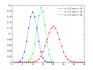
Figure - presents binomial distributions for three scenarios – two with 50% probability of success and one with a 70% probability of success and different trial sizes.

As the probability of success is varied (from 50%) the distribution will also shift its shape,becoming positively skewed for probabilities less than 50% and negatively skewed for probabilities greater than 50%.

2. Poisson distribution 

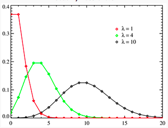
The Poisson distribution measures the likelihood of a number of events occurring within a given time interval, where the key parameter that is required is the average number of events in the given interval (l). The resulting distribution looks similar to the binomial, with the skewness being positive but decreasing with l.

 Figure - presents three Poisson distributions, with l ranging from 1 to 10.

3. Normal Distribution

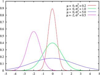
There are some datasets that exhibit symmetry, i.e., the upside is mirrored by the downside. The symmetric distribution that most practitioners have familiarity with is the normal distribution, sown in Figure - for a range of parameters:

The normal distribution has several features that make it popular. First, it can be fully characterized by just two parameters – the mean and the standard deviation – and thus reduces estimation pain. Second, the probability of any value occurring can be obtained simply by knowing how many standard deviations separate the value from the mean; the probability that a value will fall 2 standard deviations from the mean is roughly 95%. The normal distribution is best suited for data that, at the minimum, meets the following conditions:

1. There is a strong tendency for the data to take on a central value.
2. Positive and negative deviations from this central value are equally likely
3. The frequency of the deviations falls off rapidly as we move further away from the central value.

The last two conditions show up when we compute the parameters of the normal distribution: the symmetry of deviations leads to zero skewness and the low probabilities of large deviations from the central value reveal themselves in no kurtosis.

There are several more types of distributions which you can check out here.

Also, to learn about more commonly used distributions in data science check this article.