Decision Trees

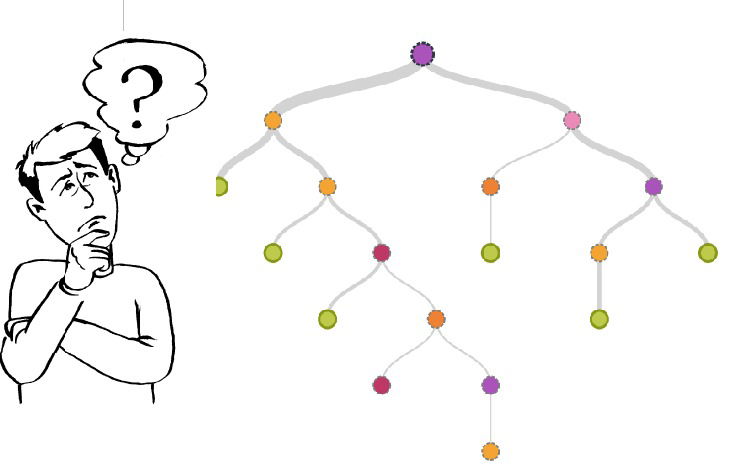
A decision tree is a decision support tool that uses a tree-like graph or model of decisions and their possible consequences, including chance event outcomes, resource costs, and utility. It is one way to display an algorithm that only contains conditional control statements.

A decision tree is a flowchart-like structure in which each internal node represents a "test" on an attribute (e.g. whether a coin flip comes up heads or tails), each branch represents the outcome of the test, and each leaf node represents a class label (decision taken after computing all attributes). The paths from root to leaf represent classification rules. Read more.

Classification And Regression Trees for Machine Learning

Decision Trees are an important type of algorithm for predictive modeling machine learning.

The classical decision tree algorithms have been around for decades and modern variations like random forest are among the most powerful techniques available.

Classification and Regression Trees or CART for short is a term introduced by Leo Breimanto refer to Decision Tree algorithms that can be used for classification or regression predictive modeling problems.

Classically, this algorithm is referred to as “decision trees”, but on some platforms like R they are referred to by the more modern term CART.

The CART algorithm provides a foundation for important algorithms like bagged decision trees, random forest and boosted decision trees.

There are two main types of Decision Trees:

1. Classification trees (Yes/No types)

Here the decision variable is Categorical, e.g. category like fit, unfit

2. Regression trees (Continuous data types)

Here the decision or the outcome variable is Continuous, e.g. a number like 123.

Associated Terms:

Entropy

Entropy, also called as Shannon Entropy is denoted by H(S) for a finite set S, is the measure of the amount of uncertainty or randomness in data.

Intuitively, it tells us about the predictability of a certain event. Example, consider a coin toss whose probability of heads is 0.5 and probability of tails is 0.5. Here the entropy is the highest possible, since there’s no way of determining what the outcome might be. Alternatively, consider a coin which has heads on both the sides, the entropy of such an event can be predicted perfectly since we know beforehand that it’ll always be heads. In other words, this event has no randomness hence it’s entropy is zero. Read more

In particular, lower values imply less uncertainty while higher values imply high uncertainty.

Information Gain

Information gain is also called as Kullback-Leibler divergence denoted by IG(S,A) for a set S is the effective change in entropy after deciding on a particular attribute A. It measures the relative change in entropy with respect to the independent variables.

Alternatively,

where IG(S, A) is the information gain by applying feature A. H(S) is the Entropy of the entire set, while the second term calculates the Entropy after applying the feature A, where P(x) is the probability of event x.

Gini Index

Gini Index is a metric to measure how often a randomly chosen element would be incorrectly identified. It means an attribute with lower gini index should be preferred.

Read more

The general motive of using Decision Tree is to create a training model which can use to predict class or value of target variables by learning decision rules inferred from prior data(training data).

Decision Tree Algorithm Pseudocode

1. Place the best attribute of the dataset at the root of the tree.
2. Split the training set into subsets. Subsets should be made in such a way that each subset contains data with the same value for an attribute.
3. Repeat step 1 and step 2 on each subset until you find leaf nodes in all the branches of the tree.

In decision trees, for predicting a class label for a record we start from the root of the tree. We compare the values of the root attribute with record’s attribute. On the basis of comparison, we follow the branch corresponding to that value and jump to the next node.

We continue comparing our record’s attribute values with other internal nodes of the tree until we reach a leaf node with predicted class value. As we know how the modeled decision tree can be used to predict the target class or the value. Now let’s understanding how we can create the decision tree model.

Assumptions while creating Decision Tree

The below are the some of the assumptions we make while using Decision tree:

1. At the beginning, the whole training set is considered as the root.
2. Feature values are preferred to be categorical. If the values are continuous then they are discretized prior to building the model.
3. Records are distributed recursively on the basis of attribute values.
4. Order to placing attributes as root or internal node of the tree is done by using some statistical approach.

Decision Tree Algorithm Advantages and Disadvantages

Advantages:

1. Decision Trees are easy to explain. It results in a set of rules.
2. It follows the same approach as humans generally follow while making decisions.
3. Interpretation of a complex Decision Tree model can be simplified by its visualizations. Even a naive person can understand logic.
4. The Number of hyper-parameters to be tuned is almost null.

Disadvantages:

1. There is a high probability of overfitting in Decision Tree.
2. Generally, it gives low prediction accuracy for a dataset as compared to other machine learning algorithms.
3. Information gain in a decision tree with categorical variables gives a biased response for attributes with greater no. of categories.
4. Calculations can become complex when there are many class labels.